
Explain and query plans.
A query that is slow is slow for a reason, and the plan is where the reason is written down. The console has a dedicated Explain page - Query → Explain in the sidebar - that runs your SQL, draws the operator tree, and points at the operator that burned the time.
The workbench once carried EXPLAIN and EXPLAIN ANALYZE buttons next to RUN. They were removed. Its action bar is now just SAVE and RUN, and its Plan results tab is a placeholder that never fills. Plans live here.
Run an explain.
- Check the instance in the top bar is the one you mean.
- Paste a
SELECTinto the SQL box. Leave theEXPLAINkeyword off - the page adds it. (If you do type it, it is not doubled up.) - Leave Analyze ticked - it is on by default - and click RUN EXPLAIN.
SELECT o.id, c.name, c.country, o.amount_cents
  FROM shop.orders o
  JOIN shop.customers c ON o.customer = c.id
 WHERE o.status = 'paid'
 LIMIT 10
With Analyze on, the engine runs the query and annotates each operator with what it actually did. That is what makes the timings real - and it also means the query does real work on the instance. Keep a LIMIT on while you are iterating, and untick Analyze if you only want the shape.
Four numbers land above the tree the moment it returns. Read them in this order: hot operator first (that is where to look), then total time (is this worth fixing), then rows returned against operator count (how much work per row of output).
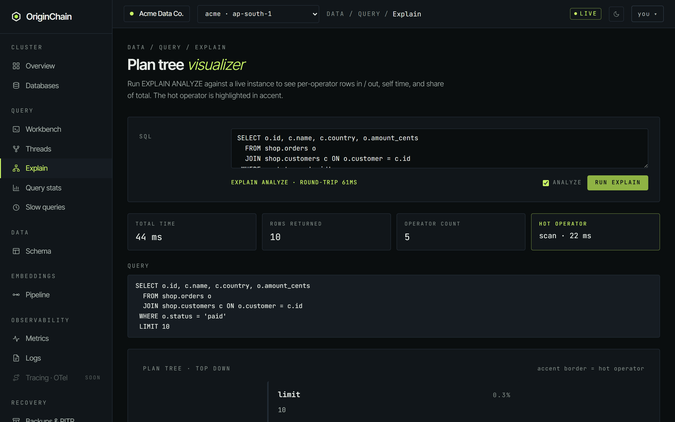
Under the strip the page echoes back the query it explained, so a tree you screenshot or share always carries the SQL it came from.
Read the plan tree.
The tree is drawn top down: the operator that produces your final rows is at the top, and its inputs hang beneath it. Data flows the other way - bottom to top - so the way to read it is to start at the leaves and work up.
The join query above produces this shape:
limit(10)
  hash_join(on customer = id)
    filter(Eq { path: "status", value: String("paid") })
      scan(shop.orders)
    scan(shop.customers)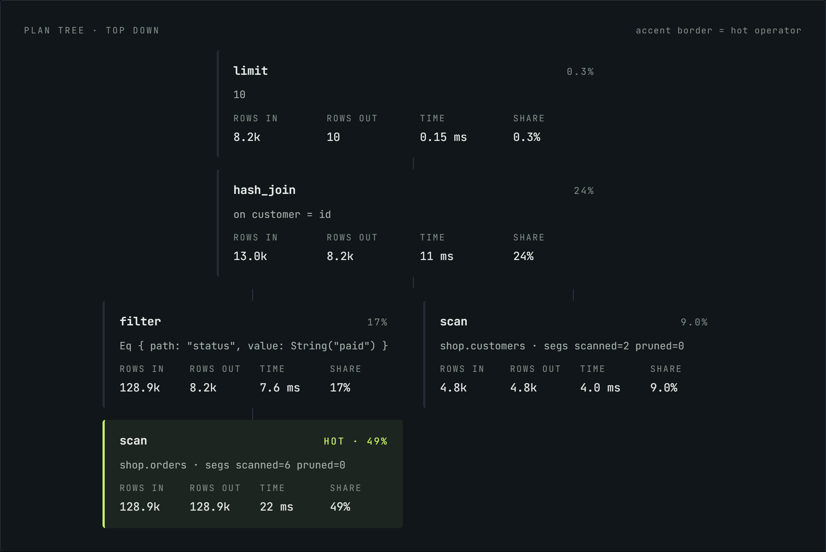
The four operators in this plan.
| Operator | What it does |
|---|---|
| scan | Reads a table. The detail line names the table and reports segs scanned and pruned - how many storage segments it had to open versus how many it managed to skip. A scan whose rows in equals its rows out read the whole table. |
| filter | Applies a predicate to the rows below it. The detail line spells out the predicate it is enforcing. Its rows-in against rows-out is the selectivity: a big drop here means the filter did useful work, but it did it after the rows were already read. |
| hash_join | Joins its two children on the equality shown in the detail line. It has two inputs, so it is the one node in this tree that branches. |
| limit | Caps the rows that leave the plan. Sitting at the top, it is usually cheap - and that is worth noticing: a LIMIT 10 does not stop the work underneath it from happening. |
Other query shapes produce other operators - the tree you get depends on what the planner chose for the query you gave it. The reading method below does not change.
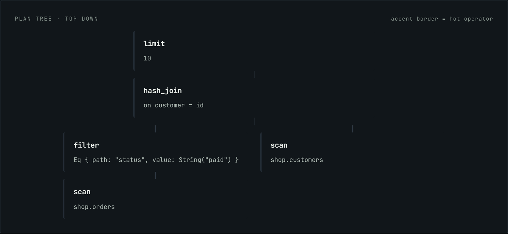
The four fields on every card.
- rows in - how many rows this operator was handed.
- rows out - how many it passed on. The gap is the work it did.
- time - self time. The console subtracts the children's time from the operator's own, so a parent is never credited with its children's cost. This is the field that makes the tree readable.
- share - that self time as a percentage of the whole plan. The shares add up to 100%.
It gets the accent border and a hot badge, and it is repeated in the header strip. It is chosen on self time, not total - which is why it lands on the leaf that is genuinely expensive rather than on whatever happens to sit nearest the top of the tree.
Structure without running it.
Untick Analyze and the engine plans the query without executing it. You get the same tree with the same operators and detail lines, but no rows, no timings, no shares - and the header strip's timing tiles show a dash. Use it when the query is expensive, or when the only thing you want to know is "did it decide to join these two the way I expected".
Query stats - what to explain in the first place.
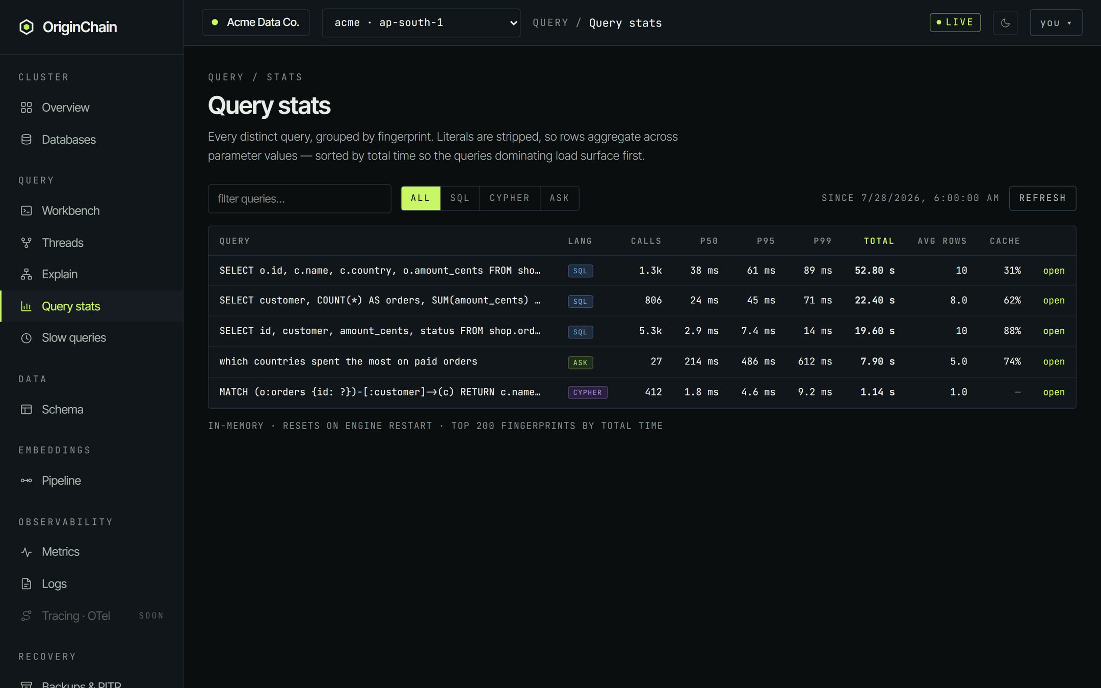
Query → Query stats aggregates every query the instance has served, grouped by fingerprint - the query with its literals replaced by ?, so a thousand runs with different parameter values collapse into one row. It is sorted by total time by default, which is exactly the right default: the query dominating your instance is rarely the slowest one, it is the merely-slow one you run constantly.
What to look for:
- total - the top row is where your instance's time goes. Start there, not at the bottom.
- p95 and p99 far above p50 - the query is usually fine and occasionally terrible. That is a different problem from "uniformly slow", and it usually means a data-dependent path: some parameter values hit far more rows than others.
- avg rows - a big average row count on a query nobody reads in full is a projection or
LIMITyou should tighten. - cache - the hit rate, where the engine reports one.
Every column header sorts, the box at the top filters by text, and the All / SQL / Cypher / Ask buttons narrow by language. open at the end of a row loads that fingerprint's page in the workbench against the same instance.
The registry lives in the engine's memory and holds the top 200 fingerprints by total time. The since timestamp on the right of the toolbar tells you how far back the numbers go - a restart resets them, so a suspiciously quiet instance may just have been restarted recently.
Slow queries - the individual runs.
Where Query stats aggregates, Query → Slow queries is the raw log: the most recent executions, newest first, with their real text and the literals intact. Drag the threshold slider up to hide everything under a given number of milliseconds - on a busy instance that is the difference between a wall of noise and the three runs you care about.
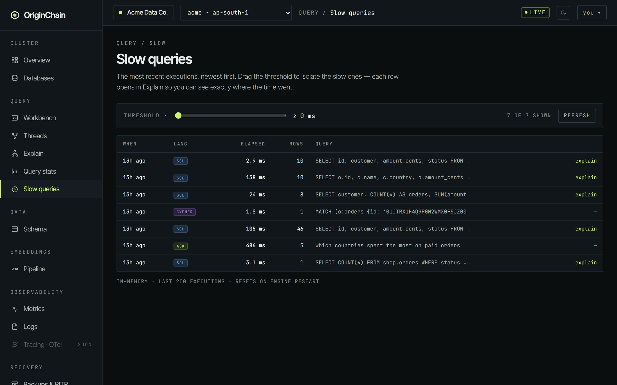
Three details that matter:
- The explain link is the whole point of the page - it opens the Explain page with that execution's SQL prefilled and already run, so you go from "this took too long" to its plan in one click.
- Only SQL rows get that link. Cypher and natural-language rows show a dash - there is no plan visualiser for them.
- Anything at or above 100 ms is called out in amber, independently of where you have the slider.
Like Query stats, this is an in-memory ring - the last 200 executions, cleared on engine restart. It is a live debugging tool, not an audit trail.
Turning a plan into a fix.
A plan tells you where the time went. What you do about it falls into two buckets: change the schema, or change the query.
Change the schema.
The signature to look for is a scan whose rows out are far larger than what the filter above it keeps. In the plan above, the scan reads every row of shop.orders and the filter immediately throws most of them away - and the scan's pruned=0 confirms it could not skip any storage segment on the way. The rows the query wanted were known up front; the engine just had no structure that let it find them without reading everything.
That is a secondary index on the filtered column. Indexes are part of the table's definition, so you add one on Data → Schema, in the table's secondary indexes section - not from the Explain page. Re-run the explain afterwards and compare: the same query should come back with a different leaf operator, and a smaller share on it.
Change the query.
- The hot operator is a join. Filter harder before the join rather than after it - anything you can move into the
WHEREof the larger side is work the join never has to do. - Rows out is much larger than what you use. Project the columns you actually need instead of everything, and make sure the
LIMITreflects what you will really read. Remember that a limit at the top of the tree does not make the work below it disappear. - p95 is far above p50 in Query stats but a one-off explain looks fine. You explained a cheap parameter value. Take a genuinely slow run from Slow queries - literals intact - and explain that one instead.
Query stats to find what costs you the most → Slow queries to grab a real slow execution of it → Explain to see which operator burned the time → change the schema or the query → explain it again and check the share moved. The Telemetry tab in the workbench closes the loop from the other end, showing the same per-fingerprint numbers next to the query you are editing.